
-
Pl
chevron_right
Erlang Solutions: Reimplementing Technical Debt with State Machines
news.movim.eu / PlanetJabber • 6 December 2023 • 16 minutes
In the ever-evolving landscape of software development, mastering the art of managing complexity is a skill every developer and manager alike aspires to attain. One powerful tool that often remains in the shadows, yet holds the key to simplifying intricate systems, is the humble state machine. Let’s get started.
Models
State machines can be seen as models that represent system behaviour. Much like a flowchart on steroids, these models represent an easy way to visualise complex computation flows through a system.
A typical case study for state machines is the modelling implementation of internet protocols. Be it TLS, SSH, HTTP or XMPP, these protocols define an abstract machine that reacts to client input by transforming its own state, or, if the input is invalid, dying.
A case study
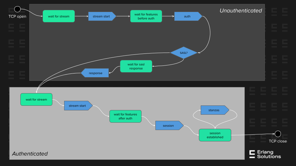
Let’s see the case for –a simplified thereof– XMPP protocol. This messaging protocol is implemented on top of a TCP stream, and it uses XML elements as its payload format. The protocol, on the server side, goes as follows:
- The machine is in the “waiting for a stream-start” state, it hasn’t received any input yet.
- When the client sends such stream-start, a payload looking like the following:
<stream:stream to='localhost' version='1.0' xml:lang='en' xmlns='jabber:client' xmlns:stream='http://etherx.jabber.org/streams'>
Then the machine forwards certain payloads to the client –a stream-start and a stream-features, its details are omitted in this document for simplicity– and transitions to “waiting for features before authentication”.
- When the client sends an authentication request, a payload looking like the following:
<auth xmlns='urn:ietf:params:xml:ns:xmpp-sasl' mechanism='PLAIN'>AGFsaWNFAG1hdHlncnlzYQ==</auth>
Then the machine, if no request-response mechanism is required for authentication, answers to the client and transitions to a new “waiting for stream-start”, but this time “after authentication”.
- When the client again starts the stream, this time authenticated, with a payload like the following:
<stream:stream to='localhost' version='1.0' xml:lang='en' xmlns='jabber:client' xmlns:stream='http://etherx.jabber.org/streams'>
Then the machine again answers the respective payloads, and transitions to a new “waiting for features after authentication”.
- And finally, when the client sends
<iq type='set' id='1c037e23fab169b92edb4b123fba1da6'>
<bind xmlns='urn:ietf:params:xml:ns:xmpp-bind'>
<resource>res1</resource>
</bind>
</iq>
Then in transitions to “session established”.
- From this point, other machines can find it and send it new payloads, called “stanzas”, which are XML elements whose names are one of “message”, “iq”, or “presence”. We will omit the details of these for the sake of simplicity again.
Because often one picture is worth a thousand words, see the diagram below:
Implementing the case
Textbook examples of state machines, and indeed the old OTP implementation of such behaviour, gen_fsm, always give state machines whose states can be defined by a single name, not taking into account that such a name can be “the name of” a data structure instead. In Erlang in particular, gen_fsm imposed the name of the state to be an atom, just so that it can be mapped to a function name and be callable. But this is an unfortunate oversight of complexity management, where the state of a machine depends on a set of variables that, if not in the name, need to be stored elsewhere, usually the machine’s data, breaking the abstraction.
Observe in the example above, the case for waiting for stream-start and features: they both exist within unauthenticated and authenticated realms. A naive implementation, where the function name is the state, the first parameter the client’s input, and the second parameter the machine’s data, would say that:
wait_for_stream(stream_start, Data#data{auth = false}) ->
	{wait_for_feature, Data}.

wait_for_feature(authenticate, Data#data{auth = false}) ->
	{wait_for_stream, Data#data{auth = true}}.

wait_for_stream(stream_start, Data#data{auth = true}) ->
	{wait_for_feature, Data}.

wait_for_feature(session, Data#data{auth = true}) ->
	{session, Data}.
In each case, we will take different actions, like building different answers for the client, so we cannot coalesce seemingly similar states into less functions.
But what if we want to implement retries on authentication?
We need to add a new field to the data record, as follows:
wait_for_stream(stream_start, Data#data{auth = false}) ->
	{wait_for_feature, Data#data{retry = 3}}.

wait_for_feature(authenticate, Data#data{auth = false}) ->
	{wait_for_stream, Data#data{auth = true}};
wait_for_feature(_, Data#data{auth = false, retry = 0}) ->
stop;
wait_for_feature(_, Data#data{auth = false, retry = N}) ->
	{wait_for_feature, Data#data{auth = true, retry = N - 1}}.
The problem here is twofold:
- When the machine is authenticated, this field is not valid anymore, yet it will be kept in the data record for the whole life of the machine, wasting memory and garbage collection time.
- It breaks the finite state machine abstraction –too early–, as it uses an unbounded memory field with random access lookups to decide how to compute the next transition, effectively behaving like a full Turing Machine — note that this power is one we will need nevertheless, but we will introduce it for a completely different purpose.
This can get unwieldy when we introduce more features that depend on specific states. For example, when authentication requires roundtrips and the final result depends on all the accumulated input of such roundtrips, we would also accumulate them on the data record, and pattern-match which input is next, or introduce more function names.
Or if authentication requires a request-response roundtrip to a separate machine, if we want to make such requests asynchronous because we want to process more authentication input while the server processes the first payload, we would also need to handle more states and remember the accumulated one. Again, storing these requests on the data record keeps more data permanent that is relevant only to this state, and uses more memory outside of the state definition. Fixing this antipattern lets us reduce the data record from having 62 fields to being composed of only 10.
Before we go any further, let’s talk a bit about automatas.
Automata theory
In computer sciences, and more particularly in automata theory, we have at our disposal a set of theoretical constructs that allow us to model certain problems of computation, and even more ambitiously, define what a computer can do altogether. Namedly, there are three automatas ordered by computing power: finite state machines, pushdown automatas, and Turing machines. They define a very specific algorithm schema, and they define a state of “termination”. With the given algorithm schema and their definition of termination, they are distinguished by the input they are able to accept while terminating.
Conceptually, a Turing Machine is a machine capable of computing everything we know computers can do: really, Turing Machines and our modern computers are theoretically one and the same thing, modulo equivalence.
Let’s get more mathematical. Let’s give some definitions:
- Alphabet: a set denoted as Σ of input symbols, for example Σ = {0,1}, or Σ = [ASCII]
- A string over Σ: a concatenation of symbols of the alphabet Σ
- The Power of an Alphabet: Σ*, the set of all possible strings over Σ, including the empty set (an empty string).
An automaton is said to recognise a string over if it “terminates” when consuming the string as input. On this view, automata generate formal languages, that is, a specific subset of Σ* with certain properties. Let’s see the typical automata:
- A Finite State Machine is a finite set of states Q (hence the name of the concept), an alphabet Σ and a function 𝛿 of a state and an input symbol that outputs a new state (and can have side-effects)
- A Pushdown Automata is a finite set of states Q, an alphabet Σ, a stack Γ of symbols of Σ, and a function 𝛿 of a state, an input symbol, and the stack, that outputs a new state, and modifies the stack by either popping the last symbol, pushing a new symbol, or both (effectively swapping the last symbol).
- A Turing Machine is a finite set of states Q, an alphabet Σ, an infinite tape Γ of cells containing symbols of Σ, and a function 𝛿 of a state, an input symbol, and the current tape cell, that outputs a new state, a new symbol to write in the current cell (which might be the same as before), and a direction, either left or right, to move the head of the tape.
Conceptually, Finite State Machines can “keep track of” one thing, while Pushdown Automata can “keep track of” up to two things. For example, there is a state machine that can recognise all strings that have an even number of zeroes, but there is no state machine that can recognise all strings that have an equal number of ones and zeroes. However,this can be done by a pushdown automaton. But, neither state machines nor pushdown automata can generate the language for all strings that have an equal number of a’s, b’s, and c’s: this, a Turing Machine can do.
How to relate these definitions to our protocols, when the input has been defined as an alphabet? In all protocols worth working on, however many inputs there are, they are finite set which can be enumerated. When we define an input element as, for example,
<stream:start to=[SomeHost]/>
, the list of all possible hosts in the world is a finite list, and we can isomorphically map these hosts to integers, and define our state machines as consuming integers. Likewise for all other input schemas. So, in order to save the space of defining all possible inputs and all possible states of our machines, we will work with
schemas
, that is, rules to construct states and input. The abstraction is isomorphic.
Complex states
We know that state machine behaviours, both the old gen_fsm and the new gen_statem, really are Turing Machines: they both keep a data record that can hold unbounded memory, hence acting as the Turing Machine tape. The OTP documentation for the gen_statem behaviour even says so explicitly:
Like most gen_ behaviours, gen_statem keeps a server Data besides the state. Because of this, and as there is no restriction on the number of states (assuming that there is enough virtual machine memory) or on the number of distinct input events, a state machine implemented with this behaviour is in fact Turing complete. But it feels mostly like an Event-Driven Mealy machine .
But we can still model a state machine schema with accuracy. ‘gen_statem’, on initialisation, admits a callback mode called ‘handle_event_function’. We won’t go into the details, but they are well explained in the available official documentation .
By choosing the callback mode, we can use data structures as states. Note again that, theoretically, a state machine whose states are defined by complex data structures are isomorphic to giving unique names to every possible combination of such data structures internals: however large of a set, such a set is still finite.
Now, let’s implement the previous protocol in an equivalent manner, but with no data record whatsoever, with retries and asynchronous authentication included:
handle_event(_, {stream_start, Host},
             [{wait_for_stream, not_auth}], _) ->
    StartCreds = get_configured_auth_for_host(Host),
    {next_state, [{wait_for_feature, not_auth}, {creds, StartCreds}, {retry, 3}]};

handle_event(_, {authenticate, Creds},
             [{wait_for_feature, not_auth}, {creds, StartCreds}, {retries, -1}], _) ->
	stop;
handle_event(_, {authenticate, Creds},
             [{wait_for_feature, not_auth}, {creds, StartCreds}, {retries, N}], _) ->
    Req = auth_server:authenticate(StartCreds, Creds),
    {next_state, [{wait_for_feature, not_auth}, {req, Req}, {creds, Creds}, {retries, N-1}]};
handle_event(_, {authenticated, Req},
             [{wait_for_feature, not_auth}, {req, Req}, {creds, Creds} | _], _) ->
    {next_state, [{wait_for_stream, auth}, {jid, get_jid(Creds)}]};
handle_event(_, Other,
             [{wait_for_feature, not_auth} | _], _) ->
    {keep_state, [postpone]};

handle_event(_, {stream_start, Host}, [{wait_for_stream, auth}, {jid, JID}], _) ->
    {next_state, [{wait_for_feature, auth}, {jid, JID}]};

handle_event(_, {session, Resource}, [{wait_for_feature, auth}, {jid, JID}], _) ->
    FullJID = jid:replace_resource(JID, Resource),
    session_manager:put(self(), FullJID),
    {next_state, [{session, FullJID}]};
And from this point on, we have a session with a known Jabber IDentifier (JID) registered in the session manager, that can send and receive messages. Note how the code pattern-matches between the given input and the state, and the state is a proplist ordered by every element being a substate of the previous.
Now the machine is ready to send and receive messages, so we can add the following code:
handle_event(_, {send_message_to, Message, To},
             [{session, FullJID}], _) ->
    ToPid = session_manager:get(To),
    ToPid ! {receive_message_from, Message, FullJID,
    keep_state;
handle_event(_, {receive_message_from, Message, From},
             [{session, FullJID}], #data{socket = Socket}) ->
    tcp_socket:send(Socket, Message),
    keep_state;
Only in these two function clauses, state machines interact with each other. There’s only one element that would be needed to be stored on the data record: the Socket. This element is valid for the entire life of the state-machine, and while we could include it on the state definition for every state, for once we might as well keep it globally on the data record for all of them, as it is globally valid.
Please read the code carefully, as you’ll find it is self-explanatory.
Staged processing of events
A protocol like XMPP, is defined entirely in the Application Layer of the OSI Model , but as an implementation detail, we need to deal with the TCP (and potentially TLS) packets and transform them into the XML data-structures that XMPP will use as payloads. This can be implemented as a separate gen_server that owns the socket, receives the TCP packets, decrypts them, decodes the XML binaries, and sends the final XML data structure to the state-machine for processing. In fact, this is how this protocol was originally implemented, but for completely different reasons.
In much older versions of OTP, SSL was implemented in pure Erlang code, where crypto operations (basically heavy number-crunching), was notoriously slow in Erlang. Furthermore, XML parsing was also in pure Erlang and using linked-lists as the underlying implementation of the strings. Both these operations were terribly slow and prone to produce enormous amounts of garbage, so it was implemented in a separate process. Not for the purity of the state machine abstractions, but simply to unblock the original state machine from doing other protocol related processing tasks.
But this means a certain duplicity. Every client now has two Erlang processes that send messages to each other, effectively incurring a lot of copying in the messaging. Now OTP implements crypto operations by binding to native libcrypto code, and XML parsing is done using exml , our own fastest XML parser available in the BEAM world. So the cost of packet preprocessing is now lower than the message copying, and therefore, it can be implemented in a single process.
Enter internal events:
handle_event(info, {tls, Socket, Payload}, _, Data#{socket = Socket}) ->
	XmlElements = exml:parse(tls:decrypt(Socket, Payload)),
	StreamEvents = [{next_event, internal, El} || El <- XmlElements],
	{keep_state, StreamEvents};
Using this mechanism, all info messages from the socket will be preprocessed in a single function head, and all the previous handlers simply need to match on events of type internal and of contents an XML data structure.
A pure abstraction
We have prototyped a state machine implementing the full XMPP Core protocol (RFC6120) , without violating the abstraction of the state machine. At no point do we have a full Turing-complete machine, or even a pushdown automaton. We have a machine with a finite set of states and a finite set of input strings, albeit large as they’re both defined schematically, and a function, `handle_event/4`, that takes a new input and the current state and calculates side effects and the next state.
However, for convenience we might break the abstraction in sensible ways. For example, in XMPP, you might want to enable different configurations for different hosts, and as the host is given in the very first event, you might as well store in the data record the host and the configuration type expected for this connection – this is what we do in MongooseIM’ s implementation of the XMPP server.
Breaking purity
But there’s one point of breaking in the XMPP case, which is in the name of the protocol. “ X” stands for extensible , that is, any number of extensions can be defined and enabled, that can significantly change the behaviour of the machine by introducing new states, or responding to new events. This means that the function 𝛿 that decides the next step and the side-effects, does not depend only on the current state and the current input, but also on the enabled extensions and the data of those extensions.
Only at this point we need to break the finite state machine abstraction: the data record will keep an unbounded map of extensions and their data records, and 𝛿 will need to take this map to decide the next step and decide not only the next state and the side-effects, but also what to write on the map: that is, here, our State Machine does finally convert into a fully-fledged Turing Machine.
With great power…
Restraining your protocol to a Finite State Machine has certain advantages:
- Memory consumption: the main difference, simplifying, between a Turing Machine and an FSM, is that the Turing Machine has infinite memory at its disposal, which means that when you have way too many Turing Machines roaming around in your system, it might get hard to reason about the amount of memory they all consume and how it aggregates. In contrast, it’s easier to reason about upper bounds for the memory the FSMs will need.
- Determinism: FSMs exhibit deterministic behaviour, meaning that the transition from one state to another is uniquely determined by the input. This determinism can be advantageous in scenarios where predictability and reliability are crucial. Turing machines instead can exhibit a complexity that may not be needed for certain applications.
- Halting: we have all heard of the Halting Problem, right? Turns out, proving that a Finite State Machine halts is always possible.
- Testing: as the number of states and transitions of an FSM are finite, testing all the code-paths of such a machine is indeed a finite task. There are indeed State Machine learning algorithms that verify implementations (see LearnLib ) and property-based testing has a good chance to reach all edge-cases.
When all we wanted was to implement a communication protocol, as varied as XMPP or TLS, where what we implement is a relationship of input, states, and output, a Finite State Machine is the right tool for the job. Using hierarchical states can model certain states better than using a simplified version of the states and global memory to decide the transitions (i.e., implement 𝛿) and will result in a purer and more testable implementation.
Further examples:
- MongooseIM’s XMPP server implementation of the client-to-server code: https://github.com/esl/MongooseIM/blob/6.1.0/src/c2s/mongoose_c2s.erl
- MongooseIM’s 6.1 release blog with details of the c2s reimplementation: https://www.erlang-solutions.com/blog/mongooseim-6-1-handle-more-traffic-consume-less-resources/
- OTP’s implementation of the SSH connection handler: https://github.com/erlang/otp/blob/OTP-26.0/lib/ssh/src/ssh_connection_handler.erl
- OTP’s implementation of TLS generic machines: https://github.com/erlang/otp/blob/OTP-26.0/lib/ssl/src/ssl_gen_statem.erl
The post Reimplementing Technical Debt with State Machines appeared first on Erlang Solutions .